LGL - the Large Graph Layout
Published:
The Large Graph Layout (LGL)
Last summer, I had a 500,000 node/million edge network, and no way to look at its structure. Cytoscape maxed out at about 100,000 edges, and for some reason which I can’t remember now, I never got my network to load on the million node capable OpenOrd Layout for Gephi.
As nicely outlined by in Martin Krzywinski’s Hive Plot page, even if a software is capable of laying out a giant network, it is more than likely to create an uninterpretable hairball. The Large Graph Layout (LGL) was created by Alex Adai in Edward Marcotte’s lab to visualize large networks while avoiding hairballs. The algorithm itself is described in the original paper, “LGL: Creating a Map of Protein Function with an Algorithm for Visualizing Very Large Biological Networks”. Basically, the algorithm first discovers disconnected clusters in the data, and then lays them out individually. LGL works radially, where each cluster begins with a seed node, and new edges are added on spheres which are force directed outwards from the existing cluster.
LGL Examples
- The Opte Project uses a minimal spanning LGL to map the internet every few years.
- Aaron Swartz used LGL for a neat visualization of blogspace in 2006.
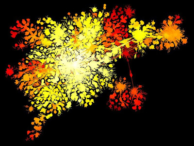
- The Museum of Modern Art in New York picked an LGL of protein homologies (top image) for their 2008 exhibit “Design and the Elastic Mind”
LGL tips
As there aren’t many resources on using the Large Graph Layout, I wanted to do a quick post on my tips for using the software. This post is meant to supplement the main FAQ and the README. LGL is mainly maintained by the Opte Project to map the internet, and the most recent version of the software can be cloned from their Github, with git clone https://github.com/TheOpteProject/LGL.git.
Note that the lgl layout implemented on igraph lays out graphs differently (and much worse IMO) than the original LGL software. Someone inspired should fix this one day.
Formatting and installation tips
After following the README instructions to install, modify line 82 in lgl.1.d3/bin/lgl.pl to the location of the LGL perls directory
use lib 'home/claire/lgl.1.D3/perls/';
Also change line 42 to the location of the lgl binary.
#For example
my $LGLDIR = '/home/claire/lgl.1.D3/bin';
Input format (.ncol)
The input format to LGL is called .ncol, which is just a space separated list of two connected nodes with an optional third column of weight.
$ cat example.ncol
node1 node2 [optional weight]
Key points for formatting the input .ncol
- Each line must be unique
- A node may connect to many other nodes
- A node cannot connect to itself
- If a line is B-A, there cannot also be a line A-B
- There can’t be blank lines
- There can’t be blanks in any column
- No header line
node1 node2
node1 node3 # OK
node1 node2 # Will cause error
node1 node1 # Will cause error
node2 node1 # Will cause error
node3         # Will cause error
              # Trailing blank line will cause error
Coloring format (.colors)
LGL allows you to color both nodes and edges. In order to color edges, each pairwise edge must have an R G B value. To color individual nodes, each node must have an R G B value. RGB values must be scaled to one 1, so just divide each number of an RGB value by 255. The rules for formatting an .ncol file apply here too, i.e. no blanks, no empty lines, no redundancy, etc.
$ cat example.edge.colors
node1 node2 1.0 0.5 0.0
node3 node4 0.0 1.0 0.8
node5 node6 0.1 0.1 1.0

$ cat example.vertex.colors
node1 1.0 0.8 0.0
node2 1.0 0.5 0.0
node3 0.2 0.1 0.8
node4 0.0 1.0 0.8
node5 0.6 0.5 0.5
node6 0.1 0.1 1.0
An LGL workflow
This is any example to make a network with colored nodes and edges. I would begin by making a file of all pairwise edges and their associated traits. It can be difficult to keep .ncol and .color files in sync, and so it will cause fewest headaches to begin with one file containing all the information to create both.
$ echo "Nodes and traits"
$ cat homology.txt
node1 node2 source score rank species1 species2
protein1 protein2 blastp 150 1 mouse human
protein3 protein4 blastp 50 2 wheat rat
protein2 protein5 hmmscan 60 3 human human
Then take the first two columns (minus the header) to create an .ncol file. This is the file used to layout the graph
$ echo "Get node columns, remove header"
$ awk '{print $1, $2}' homology.txt  | awk '{if(NR>1)print}' > homology.ncol
$ cat homology.ncol
protein1 protein2
protein3 protein4
protein2 protein5
Then choose a trait, and create a edge.colors file. I generally select the first two columns, and a trait to color by, then just use sed to replace the trait values with the RGB value I want to color that type of edge by.
In this file, I want to color all edges predicted with the algorithm hmmscan red, and all edges found with blastp blue.
$ echo "Get node columns and trait column"
$ awk '{print $1, $2, $3}' homology.txt  | awk '{if(NR>1)print}' >  homology_alg.colors.tmp

$ echo "Replace hmmscan trait with RGB value
$ sed -i 's/hmmscan/0 1 0/g' homology_alg.colors.tmp

$ echo "Replace blastp trait with RGB value
$ sed 's/blastp/0 0 0/g' homology_alg.colors.tmp > homology_algorithm.edge.colors

$ cat homology_algorithm.edge.colors
protein1 protein2 0 0 0
protein3 protein4 0 0 0
protein2 protein5 0 1 0
I could also color each node by some trait. In this file format, each vertex must have an associated RGB value. In this case, I want to color every human protein red, and proteins from every other species blue.
$ echo "Get first column of nodes and species"
$ awk '{print $1, $6}' homology.txt  | awk '{if(NR>1)print}'> vertex1_species.tmp

$ Get second column of nodes and species"
$ awk '{print $2, $7}' homology.txt  | awk '{if(NR>1)print}'> vertex2_species.tmp

$ Get unique nodes"
$ cat vertex1_species.tmp vertex2_species.tmp | sort -u > homology_human.vertex.colors.tmp

$ Color human nodes red"
$ sed -i 's/human/1 0 0/' homology_human.vertex.colors.tmp

$ Color any other node blue"
$ sed 's/mouse\|wheat\|rat/0 0 1/' homology_human.vertex.colors.tmp > homology_human.vertex.colors

$ cat homology.human.vertex.colors
protein1 0 0 1
protein3 0 0 1
protein2 1 0 0
protein4 0 0 1
protein5 1 0 0
Running LGL
I put all the above files in one folder, /homologyLGL. This folder will also be the destination for generated LGLs. Navigating to the lgl.x.x/ directory, modify the following options in the conf_file for a particular run.
#Locations of the folder for this run, and the .ncol file
tmpdir = 'home/claire/homologyLGL'
inputfile='home/claire/homologyLGL/homology.ncol'

#Generate a full LGL, not just the minimal spanning tree (MST)
treelayout = '1'
usemst = '0'
outputmst = '0'
#No edgeweight, so:
useoriginalweights = '0'
Then just run lgl. The -c options signifies that you’re using a config file
$ ./bin/lgl.pl -c conf_file_homology
It took about 5 seconds to create my 3 line network, but it can take hours depending on the size of the network/speed of the computer. In ~/homologyLGL/, a folder 1455579482/ now contains all individual discrete subnetworks of the LGL
ls | head -5
0.lgl                #Network Layout
0.coords             #Node coordinates
0.coords.mst.lgl     #Minimal spanning tree network layout
0.coords.log         #Subnetwork measurements
0.coords.root        #Node used to root an individual subnetwork
0.coords.edge_levels #Levels of the subnetwork
~/homologyLGL/ now also contains
homology.lgl  #The complete network layout, created from the arrangement of the subnetworks
final.coords  #Node coordinates
final.mst.lgl #The minimal spanning tree version of the network layout
In order to view the LGL, run the lglview.jar program
java -jar ~/lgl.1.D3/lglview.jar
Load the lgl, and the node coordinates (File > Open .lgl file > homology.lgl, File > Open 2D coords file > final.coords)
Load the node colors to color all human proteins red and all others blue (File > Open Vertex Color File > homology.algorithm.vertex.colors) and the edge color file to color all the edges predicted with hmmscan green, and with blastp black (File > Open Edge Color File > homology.human.edge.colors). I changed the node size too, since the default is small.
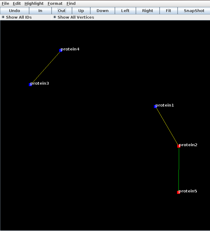
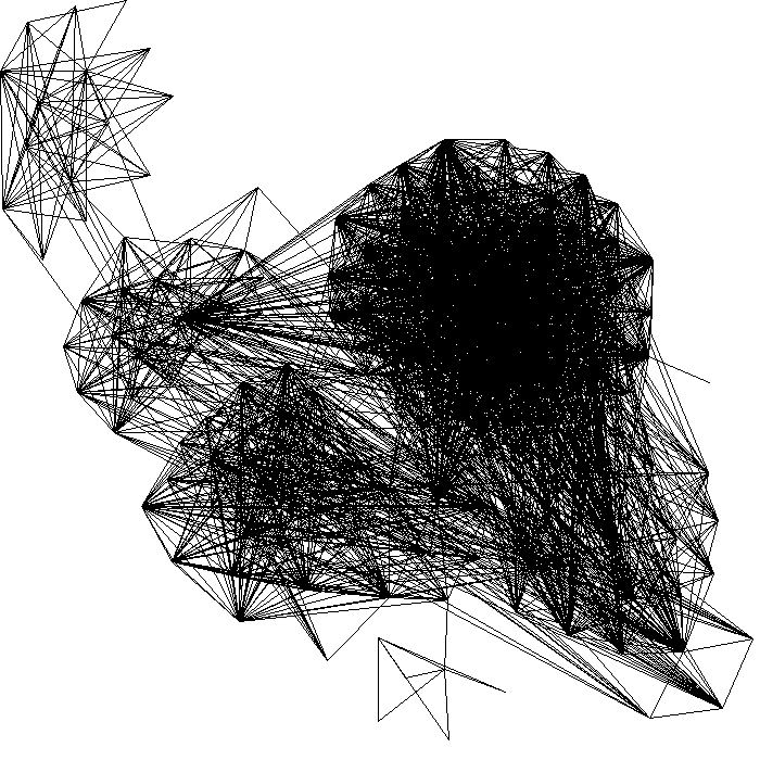
Here’s a prettier image from lglview.jar of protein families in different species linked by predictions of orthology. This network shows good separation between the fairly densely connected submodules.
High quality images
Use imageMaker.jar
cd ~/homologyLGL/
#imageMaker.jar arguments: ImageWidthInteger ImageHeightInteger edges.lgl coords1 coords2.
#If you have a file named "color_file" in the current directory
#It will read that in as an edge color file. By default edges are white.

#copy edge.colors file into filename color_file
cp homology_algorithm.edge.colors color_file

java -jar ~/lgl.1.D3/Java/imageMaker.jar 800 800 homology.lgl final.coords
Conclusion
Any type of pairwise data can be quickly formatted for LGL for a quick visual diagnostic of the data structure. Since this layout has been so useful for me to look at my data, I hope these tips will encourage others to try it out for their giant network visualization issues!
Errors I’ve run across
This error means line 82 in lgl.1.d3/bin/lgl.pl that points to the perl directory is a location that doesn’t exist
cmcwhite@claire:~/Programs/lgl.1.D3$ ./bin/lgl.pl -c conf_file
Can't locate ParseConfigFile.pm in @INC (you may need to install the ParseConfigFile module) (@INC contains: /home/clare/Programs/lgl.1.D3/perls/ /etc/perl /usr/local/lib/perl/5.18.2 /usr/local/share/perl/5.18.2 /usr/lib/perl5 /usr/share/perl5 /usr/lib/perl/5.18 /usr/share/perl/5.18 /usr/local/lib/site_perl .) at ./bin/lgl.pl line 82.
:format(webp)/cdn.vox-cdn.com/uploads/chorus_image/image/54613965/IMG_3125.0.jpg)